The schedule-adjusted league table
In most soccer leagues, the league table is the standard way to rank teams, and is used at the end of the season to crown champions and choose teams for promotion and relegation, as well as qualification for international competitions. League points are gained by winning or drawing games. However, the table does not take into account the difficulty of opponents; winning against the strongest team in the league is worth as many points as winning against the weakest. As a consequence, the schedule of when teams play each other can skew the ranking of teams in favor of those with easier schedules. This is more of a problem towards the beginning of the season. As a side note, the question of how to rank teams is more pertinent in systems where not everyone plays each other, for example the NBA.
The schedule-adjusted league table (SALT) was proposed by Constantinos Chappas as a better way to tell how well teams have been doing so far. Basically, for each pair of teams, SALT takes into account the difference in points they have gained from equivalent matchups at the equivalent venue. In doing so, it automatically considers schedule difficulty, and may therefore represent a better ranking of teams than the regular league table.
SALT uses a linear model: \(M P = R\), where \(M\) is a 190*20 matrix of every matchup times every team, \(R\) is a 190-vector of relative points, so the difference in points per game for the games that both teams have played, and \(P\) is a 20-vector of how many more points per game the team earns compared to average (will be scaled to points later), to be solved for with least-squares. For additional details, check the original post by Chappas.
SALT has some attractive properties:
- The average of the SALT points is equal to the average of the actual points after each matchday.
- At the end of the season, SALT and the actual league table are identical!
Let’s code this model up in R, and look at some results for the 2018-2019 Serie A season:
# load some packages
library(jsonlite)
library(dplyr)
library(ggplot2)
library(gganimate)
theme_set(theme_bw())

# get the data from https://github.com/openfootball/football.json
url.clubs = 'https://raw.githubusercontent.com/openfootball/football.json/master/2018-19/it.1.clubs.json'
url.results = 'https://raw.githubusercontent.com/openfootball/football.json/master/2018-19/it.1.json'
it.teams = fromJSON(url.clubs)$clubs
n.teams = nrow(it.teams)
# let's add team codes for Frosinone and SPAL
it.teams[19,2]='FRO'
it.teams[20,2]='SPA'
it.results = fromJSON(url.results)$rounds$matches
n.rounds = length(it.results)

# start by creating M matrix
create.matchup.index.matrix = function(n.teams){
  M = matrix(0, nrow=n.teams*(n.teams-1)/2, ncol=n.teams)
  i.row = 1
  for (i1 in 1:(n.teams-1)){
    for (i2 in (i1+1):n.teams){
      M[i.row, i1] = 1
      M[i.row, i2] = -1
      i.row = i.row + 1
    }
  }
  return(M)
}
M = create.matchup.index.matrix(n.teams)
To calculate \(R\), I will use two helper matrices: one 20*40 matrix of points gained per match, and another matrix with the same dimensions containing the matchday when the game took place. Each matrix contains one row per team, and one column per matchup, so 20 opponents at home plus 20 opponents away. Using these helper matrices, we can easily see which opponents two teams have played in common, which we’ll need to calculate SALT.
# create matrices to record round and points for each game
game.points = matrix(0, nrow=n.teams, ncol=2*n.teams,
  dimnames=list(it.teams$code, c(it.teams$code, it.teams$code)))
# use Inf so a team never plays itself
game.matchday = matrix(Inf, nrow=n.teams, ncol=2*n.teams,
  dimnames=list(it.teams$code, c(it.teams$code, it.teams$code)))

# create vector to translate team name to
# index, like a dictionary
name.to.index = 1:n.teams
names(name.to.index) = it.teams$name

# fill in matchday and points matrices
for (i.round in 1:n.rounds){
  current.round = it.results[[i.round]]
  n.games = nrow(current.round)

  for (i.game in 1:n.games){
    team1.index = name.to.index[current.round$team1[i.game]]
    team2.index = name.to.index[current.round$team2[i.game]]

    # record info on when game was played
    game.matchday[team1.index, team2.index] = i.round
    # add n.teams because game is away for team2
    game.matchday[team2.index, team1.index + n.teams] = i.round

    # translate scoreline to points
    # first extract score for each team
    score.team1 = current.round$score[i.game,][[1]][1]
    score.team2 = current.round$score[i.game,][[1]][2]

    # then translate to points for the game
    if (score.team1 > score.team2){
      points.team1=3
      points.team2=0
    } else if (score.team1 < score.team2){
      points.team1=0
      points.team2=3
    } else {
      points.team1=1
      points.team2=1
    }

    game.points[team1.index,
                team2.index] = points.team1
    # add n.teams because game is away for team2
    game.points[team2.index,
                team1.index + n.teams] = points.team2
  }
}

# create function to fill in R
create.relative.point.matrix = function(games.played,
                                        points.so.far){
  n.teams = nrow(points.so.far)
  R = rep(0, n.teams*(n.teams-1)/2)

  index = 1
  for (i1 in 1:(n.teams-1)){
    for (i2 in (i1+1):n.teams){
      # which games have both teams played
      games.played.in.common = (games.played[i1,] &
                                games.played[i2,])
      n.games.in.common = sum(games.played.in.common)

      # only calculate R[index] if they have matches in common
      if (n.games.in.common > 0){
        # how many points did they get from those games
        points1 = sum(points.so.far[i1, games.played.in.common])
        points2 = sum(points.so.far[i2, games.played.in.common])

        # the difference per game is R
        R[index] = (points1 - points2) / n.games.in.common
      }

      # add points for head to head matches
      if (games.played[i1, i2]){
        R[index] = R[index] *
          n.games.in.common/(n.games.in.common + 1) +
          (points.so.far[i1, i2] -
            points.so.far[i2, i1+n.teams])/(n.games.in.common + 1)
        n.games.in.common = n.games.in.common + 1
      }
      if (games.played[i1, i2 + n.teams]){
        R[index] = R[index] * n.games.in.common/
          (n.games.in.common + 1) +
          (points.so.far[i1, i2+n.teams] -
           points.so.far[i2, i1])/(n.games.in.common + 1)
        n.games.in.common = n.games.in.common + 1
      }

      index = index + 1
    }
  }
  return(R)
}
To obtain the least-squares solution, I could use lsfit, but in this case I use the Moore-Penrose pseudoinverse (via SVD) instead.
# solve linear system AX=Y with Moore-Penrose pseudoinverse
mp.solve = function(A, Y, tol=1e-8){
  svd.res = svd(A)

  # create diagonal matrix with inverse of
  # all singular values greater than tol
  sv.inv = rep(0, length(svd.res$d))
  sv.inv[svd.res$d>tol] = 1/svd.res$d[svd.res$d>tol]
  sv.mat = diag(sv.inv)

  # create pseudoinverse
  A.inv = svd.res$v %*% sv.mat %*% t(svd.res$u)

  # solve system
  X = A.inv %*% Y
  return(X)
}

# and a function to calculate P, then scale to points
calculate.adjusted.points = function(M,
                                     R,
                                     game.points,
                                     games.played,
                                     i.round){
  # use MP pseudoinverse to solve linear system
  P = mp.solve(M, R)

  # scale to points
  avg.points = mean(game.points[games.played])
  salt.points = i.round * (avg.points + P)

  return(salt.points)
}
Now, let’s calculate the actual and adjusted league points after each matchday
# create data frame with actual and schedule-adjusted points
# start with zeros
df.salt=NULL
for (i.team in 1:n.teams){
  team = it.teams$code[i.team]
  df.salt = rbind(df.salt, data.frame(team=team, matchday=0,
    actual.points=0, salt.points=0))
}

# then calculate SALT for all rounds
for (i.round in 1:n.rounds){
  games.played = game.matchday <= i.round

  points.so.far = matrix(0, nrow=n.teams, ncol=2*n.teams)
  points.so.far[games.played] = game.points[games.played]

  # fill in R matrix
  R = create.relative.point.matrix(games.played, points.so.far)

  # calculate adjusted points
  salt.points = calculate.adjusted.points(M, R, game.points,
    games.played, i.round)

  # fill in data frame
  for (i.team in 1:n.teams){
    team = it.teams$code[i.team]
    actual.points = sum(points.so.far[i.team,])
    df.salt = rbind(df.salt,
                    data.frame(team=team,
                               matchday=i.round,
                               actual.points=actual.points,
                               salt.points=salt.points[i.team]))
  }
}
Some notes on this:
avg.pointschanges with each matchday; this is so that SALT on an ongoing season will exactly match the SALT for the corresponding matchday once the full season results are in. In other words, SALT for a matchday won’t change based on how far along a season has come.- Unlike regular league points, SALT can decrease from one matchday to the next, depending on other teams’ results.
Okay, so now we have the SALT points for each matchday. Let’s start by seeing when each team had the biggest difference between actual points and adjusted points:
df.salt %>% group_by(team) %>%
  mutate(abs.diff = abs(salt.points-actual.points))
  %>% slice_max(n=1,order_by=abs.diff) %>% ungroup()
| team | matchday | actual.points | salt.points | abs.diff |
|---|---|---|---|---|
| ATA | 10 | 12 | 10.11 | 1.89 |
| BOL | 13 | 11 | 8.96 | 2.04 |
| CAG | 17 | 17 | 19.06 | 2.06 |
| CHI | 6 | 2 | 4.70 | 2.70 |
| EMP | 18 | 16 | 12.68 | 3.32 |
| FIO | 13 | 18 | 15.85 | 2.15 |
| FRO | 11 | 6 | 1.24 | 4.76 |
| GEN | 8 | 12 | 8.63 | 3.37 |
| INT | 11 | 25 | 27.92 | 2.92 |
| JUV | 3 | 9 | 6.10 | 2.90 |
| LAZ | 13 | 23 | 25.48 | 2.48 |
| MIL | 15 | 26 | 28.70 | 2.70 |
| NAP | 26 | 56 | 60.15 | 4.15 |
| PAR | 10 | 13 | 8.95 | 4.05 |
| ROM | 8 | 14 | 12.20 | 1.80 |
| SAM | 11 | 15 | 17.92 | 2.92 |
| SAS | 9 | 14 | 17.65 | 3.65 |
| SPA | 9 | 12 | 16.30 | 4.30 |
| TOR | 21 | 30 | 32.64 | 2.64 |
| UDI | 15 | 13 | 14.87 | 1.87 |
So the difference between regular and schedule-adjusted league points is always less than 5 points for the 2018-2019 Serie A season.
And how do the actual points compare with adjusted points for each matchday? Let’s plot it!
animate.salt = function(df,
                        fps=4,
                        seconds.per.round=1.5,
                        width=720,
                        height=720){
  points.min = min(min(df.salt$actual.points),
    min(df.salt$salt.points))
  points.max = max(max(df.salt$actual.points),
    max(df.salt$salt.points))
  p.anim = ggplot(data=df.salt,
    aes(x=actual.points,
      y=salt.points,
      label=team,
      color=team)) +
    geom_label(size=8) +
    geom_abline(slope=1, color='#a6a6a6') +
    labs(title='Schedule-adjusted league points',
         x='Actual league points',
         y='Schedule-adjusted points') +
    xlim(points.min, points.max) +
    ylim(points.min, points.max) +
    theme(legend.position="none",
          text = element_text(size=24)) +
    transition_states(matchday,
                      transition_length = 2,
                      state_length = 1) +
    ease_aes('cubic-in-out') +
    ggtitle('Matchday {closest_state}')

  animate(p.anim,
          nframes=(n.rounds+1)*seconds.per.round*fps,
          fps=fps,
          end_pause=6*fps,
          width=width,
          height=height)
}

animate.salt(df.salt, fps=10)
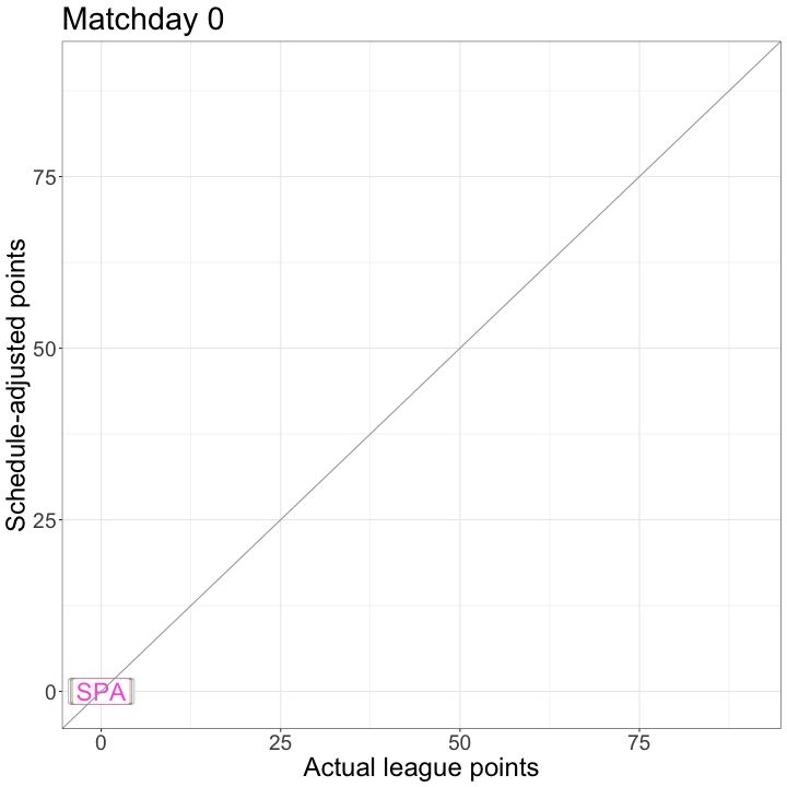
A team above the diagonal line is perhaps lower in the league table than performances merit due to a difficult schedule. Conversely, a team below the diagonal has many difficult matchups to come, and may thus drift down the league table in the future.
So that’s the schedule-adjusted league table: a more nuanced way of looking at the results so far. This is just a simple adjustment, but the model can certainly be extended by looking at recent team form, more advanced metrics like expected goals, and so on. For some other alternative league tables, take a look at:
- alt-3.uk and their methodology
- fivethirtyeight and their methodology